Bean Machine
Member
- Local time
- Today, 07:55
- Joined
- Feb 6, 2020
- Messages
- 102
Hi All,
I am struggling with finding the best way to set up this formula in Excel. Essentially what I want to do is to check the left 2 characters in cell B28 of my worksheet titled "Data" and see if there are any matches with values in range B1:AH1 of my worksheet titled "Calculations", and, if there is a match, make the cell value equal to whatever is beneath the match found in the "Calculations" worksheet. The following are some images to hopefully help in visualizing what I am talking about doing (apologies for the funky censorship job I did).
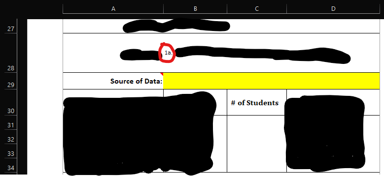
This is in the Data worksheet. I want to pull that value of "1a" and check to see if it exists in the Calculations sheet range B1:AH1

This is in the Calculations worksheet. See that there is a match to "1a" here. Now that a match has been found in range B1:AH1 I want the value below the match, in this case "0".

Imagine that beneath the "# of Students" column the "0" value appeared after the formula did its thing. This is what I ultimately want. I hope this makes sense, if not I can clarify on anything. Thank you for your time and support I hope you all have a great day.
I am struggling with finding the best way to set up this formula in Excel. Essentially what I want to do is to check the left 2 characters in cell B28 of my worksheet titled "Data" and see if there are any matches with values in range B1:AH1 of my worksheet titled "Calculations", and, if there is a match, make the cell value equal to whatever is beneath the match found in the "Calculations" worksheet. The following are some images to hopefully help in visualizing what I am talking about doing (apologies for the funky censorship job I did).
This is in the Data worksheet. I want to pull that value of "1a" and check to see if it exists in the Calculations sheet range B1:AH1
This is in the Calculations worksheet. See that there is a match to "1a" here. Now that a match has been found in range B1:AH1 I want the value below the match, in this case "0".
Imagine that beneath the "# of Students" column the "0" value appeared after the formula did its thing. This is what I ultimately want. I hope this makes sense, if not I can clarify on anything. Thank you for your time and support I hope you all have a great day.
